Excel Wizardry Unleashed: Top Tips You Need to Know

Are you ready to level up your Excel skills and become a master?

Whether you're just starting out with Excel or consider yourself an expert, these ingenious tips and tricks are about to change the game for you. Say goodbye to monotonous tasks and welcome a boost in productivity. These clever shortcuts will empower you to achieve more in less time.

Let's dive in and unlock the full potential of Excel!

This blog is an excerpt of a recent webinar.
Don't want to read the article? Watch the full recording below.

Be sure to register here for the "Getting the Most Out of Micrososft for Business" Lunch & Learn series!

• The Magic Behind Excel
• Keyboard Shortcuts
• Conditional Formatting
• Pivot Tables
• VLOOKUP Function
• Data Validation
• Sparklines 
• Excel Training
• Making the Most of Excel!

The Magic Behind Excel: It’s More Than Just Spreadsheets!

Excel is an incredibly powerful software program that empowers users to effectively manage and analyze large amounts of data. With its wide range of features, Excel not only saves professionals valuable time but also enhances efficiency and creates polished and professional-looking documents.

In order to fully harness the potential of Excel, it is crucial to develop a solid understanding of how the program works and master some essential tips and tricks to optimize your workflow.

Here are a few basics to get you started:

• To improve your Excel skills, avoid using volatile formulas that recalculate with every change. Instead, use non-volatile formulas like SUM or AVERAGE.
• Utilize tables to prevent calculation errors and add extra rows and columns for data stability.
• And finally, speed up your work with keyboard shortcuts like ALT + key combinations.

Read on to learn more!

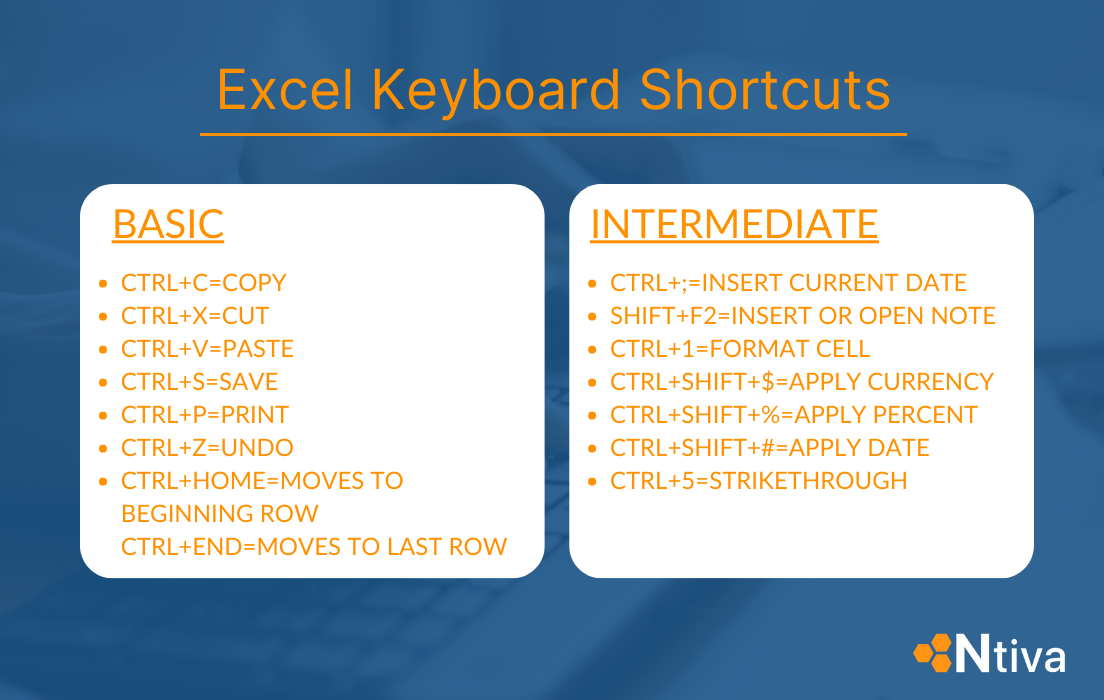
Tip #1: Use Excel Shortcuts To Speed Up Your Workflow

If you're looking to optimize your workflow and save valuable time while working with Excel, mastering keyboard shortcuts is essential. Whether you're managing personal finances or analyzing complex data sets, these shortcuts can significantly speed up your tasks. To make things even more convenient, you can customize your QAT (Quick Access Toolbar) with your preferred shortcuts, making them easily accessible every time you open Excel.

One of the most useful Excel shortcuts is quickly seeing the sum of a selected group of cells without inserting a formula. Simply select the first cell, hold down "Ctrl," and then select any other cells you want to add together. The total will appear in the bottom status bar.

On top of the time-saving shortcuts mentioned above, Excel has even more cool features to boost your workflow. For instance, you can effortlessly hide rows and columns in your spreadsheet to tidy up the layout and make it easier to read. This comes in handy, especially when dealing with hefty amounts of data.

Excel also offers the nifty capability to create hyperlinks to other sheets, cells, or even specific text within a worksheet. This feature comes in handy when dealing with cross-referenced data scattered across multiple sheets or workbooks. By taking advantage of hyperlinks, you can effortlessly navigate between different sections of your spreadsheet and streamline your data analysis process.

Looking for more Excel keyboard shortcuts?  Here you go!

Tip #2: Conditional Formatting: Highlight What Truly Matters

If you are working with a dataset that includes both text and numbers, it can be difficult to see which values stand out. This is where conditional formatting can help you.

With a few clicks, you can highlight cells or entire rows or columns of data. You can also use the color options in this tool to differentiate between different values. For example, you can format cells to display red if the number is greater than 100 or green if it is less than 10.

In addition to pre-set formats, you can also use conditional formatting to highlight data that meets specific criteria, such as the top ten items, bottom ten items, or cells above or below average. You can even create a rule that highlights cells based on a formula.

To define a custom rule in Excel's conditional formatting feature, follow these steps:

1. Select the cell or group of cells intended for formatting.

2. Go to the Home tab, then choose Conditional Formatting > New Rule.

3. In the Rule Type menu, select ‘Use a formula' to determine which cells to format.

By defining custom rules in Excel's conditional formatting, you can highlight specific cells or groups of cells based on your own criteria. This can make it easier to identify important data or patterns in your spreadsheet and improve the visual clarity of your data analysis.

Tip #3: Master Excel's Most Powerful Tool: Pivot Tables

Pivot tables are Excel's most powerful tool for making sense of large sets of data. They allow you to summarize information in columns and rows without having to create multiple individual summaries in different parts of the spreadsheet. You can also use Pivot Tables to create simple calculations, which are often a time-consuming process in other types of spreadsheets.

Here is how to create a pivot table:

1. Click anywhere in the table layout of your source data worksheet. You'll see a field list pane on the right side of your screen with four areas (Rows, Columns, Values, and Filters). Click the Recommended Pivot Table Layout to select it.
2. To add a field to the layout, drag it from the field list into one of the areas of the Pivot Table. For example, if you want to show the total sales for a specific region, drag the Region field into the Rows area.
3. Excel will automatically update the pivot table in your worksheet. If you want to remove a field from the layout, clear its check box in the Field List panel.

Tip #4: Unlock Excel's VLOOKUP Potential

The strength of VLOOKUP lies in its ability to associate two sets of data. For example, imagine you have a list of employee IDs in one column and their corresponding names in another. If you wanted to find out a name based on an employee ID, VLOOKUP would be your go-to.

Here's how to use the VLOOKUP Syntax:

To use VLOOKUP, the syntax is as follows: =VLOOKUP(lookup_value, table_array, col_index_num, [range_lookup])

1. lookup_value: The value you want to search for.

2. table_array: The range of cells containing the data you're searching through.

3. col_index_num: The column index number from which the matched value will be returned. If it's the 3rd column in your table_array, you'd enter 3.

4. [range_lookup]: This is optional. Enter FALSE for an exact match and TRUE for an approximate match. If omitted, TRUE is the default.

Remember, it always searches the first column and sort data in ascending order when using an approximate match. Understanding VLOOKUP enhances data retrieval efficiency.

Tip #5: Know The "Rules" Of Data Validation

Data validation is a powerful tool that allows you to control the type of information entered into your Excel cells. It ensures that numbers are formatted correctly, dates are in the right format, and text values are within the desired character length.

To set up a data validation rule, simply select the cell or range of cells you want to check. Then, navigate to the Data tab and click on the New Data Validation rule button.

In the window that appears, you have the option to define the criteria for validation. You can choose to allow values that match your criteria or show an error alert when invalid data is entered. The error alert gives users the choice to continue entering data, edit the current entry, or delete it. You can even create a list of acceptable responses, which is useful for situations where users need to choose from a long list of options, such as exam center locations.

Regularly using data validation not only ensures data integrity but also makes data analysis easier and more accurate. By taking the time to set up these rules, you can maintain a high-quality dataset that you can trust. Remember, garbage in equals garbage out.😉

Tip #6: Use Sparklines To Add Sizzle To Your Spreadsheet

Sparklines are a fantastic feature that adds a touch of magic to your Excel spreadsheets. These compact, in-cell charts allow you to easily visualize data patterns without the need for complex graphs. They are especially useful for creating concise and clear reports and dashboards.

To use sparklines, simply select the cell where you want to add or customize your sparkline. Then, open the 'Create Sparklines' dialog box and select the Line option. Excel even allows you to customize your sparklines with different colors, weights, and corresponding dates.

In a nutshell, sparklines are a powerful tool for effortlessly visualizing data trends directly within your spreadsheet. They provide a simplified way to understand your data, making it feel like you have a data visualization expert right at your fingertips!

Tip #7: Gain True Mastery With Microsoft Excel e-Training

If you're serious about taking your e-training to the next level, Microsoft has got you covered with a comprehensive Excel curriculum. To get started, simply head over to the Office 365 section of your Microsoft dashboard. There, you'll find a treasure trove of courses like Excel Essential Training, Excel Power Training, and Excel Pros. These modules together offer nearly 12 hours of intense Excel instruction that will supercharge your skills.

For those aiming to become true Excel power users, the Excel Power Users module is the real deal. It delves into complex operations like merging tables and expertly managing table sets. You'll also explore advanced functionalities like VLOOKUPs and discover the magic of the match function, which is a game-changer when working with extensive data matrices. It takes the conventional VLOOKUP to a whole new level of sophistication.

Armed with these incredible resources, you'll be ready to wow organizational leadership with your superior data presentations and analyses. Excel is an indispensable tool in the modern business world, and our training ensures that you'll make the most of its capabilities. So get ready to excel like never before!

PRO TIP: Register for our monthly training on all things Microsoft here! 

Summary: Making the Most of Excel!

In a nutshell, Excel in Microsoft 365 is a treasure trove of resources that will take your data presentation to the next level. It empowers users to effortlessly analyze and visualize data, making it a must-have tool for professionals. With Excel's power at your fingertips, you can confidently manage and present data in a captivating and impactful manner, unlocking endless possibilities for efficient data management and presentation.

Get ready to dazzle your audience like never before!